Interpretable ML
约 1400 个字 预计阅读时间 5 分钟
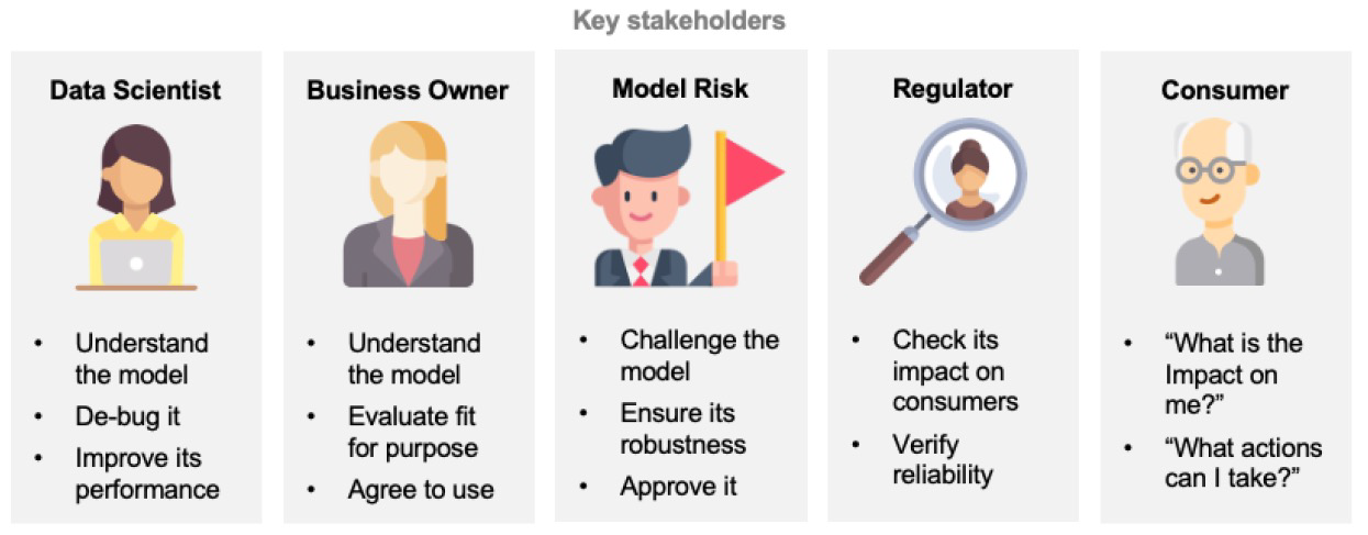
Challenges
- Do we understand the decisions suggested by ML models?
- Can we trust ML models if their decision-making process is not fully transparent?
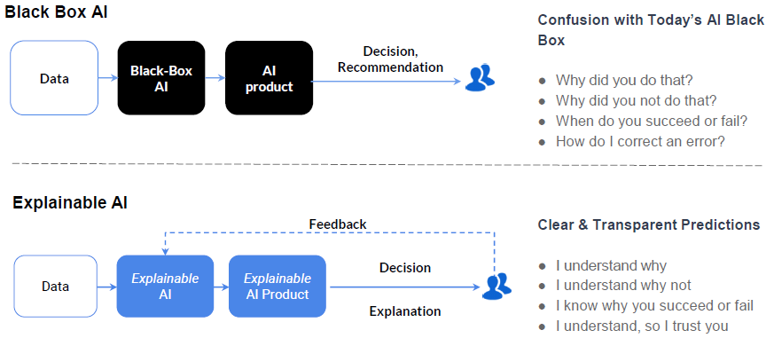
Explainable ML refers to methods and techniques in the application of ML systems such that the results of the solution can be understood by human experts and users
transparent models & opaque models
Feature relevance (or feature attribution) is also applied with non-image data for quantifying the influence of each input variable toward the model decision
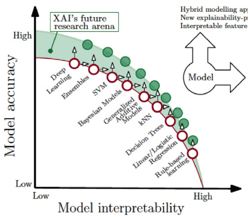
Currently, the best performing models in terms of accuracy are the least interpretable
Pixel level
!!! note "which input pixels are important when a model classifies one input example? (Local Explanation)"
Vanilla BackProp
The approach uses backpropagation to visualize the gradients with respect to each pixel of an image
Guided BackProp
Occlusion Maps
Systematically occlude different portions of the input image with a grey square, and monitor the output of the classifier
E.g., in the image, the strongest feature is the dog’s head - Occlusion maps is an older and computationally expensive method

CAM
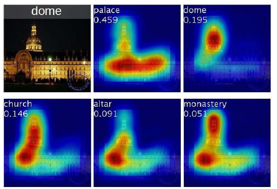
CAM produces a heatmap for the pixels that activate the most model’s prediction of a specific class of objects
Grad-CAM
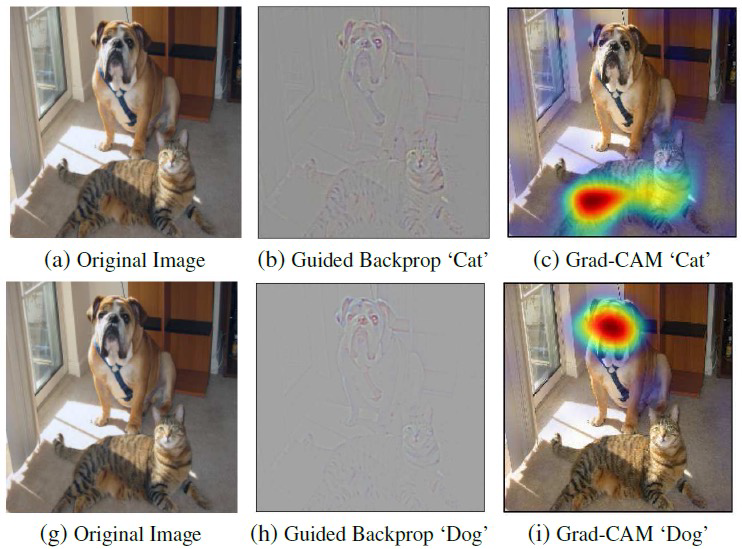
Grad-CAM is an extension of the CAM approach
- It employs gradient backpropagation to improve the heatmaps
- Compare Grad-CAM to Guided BackProp for the classes ‘Cat’ and “Dog’ in the image
Guided Grad-CAM
Integrated Gradients
Integrated gradients employs the integral of the gradients of a black-box model \(F\) along a straight-line path from a baseline input \(z\) to an input instance \(x\)
LRP
Layer-wise Relevancy Propagation
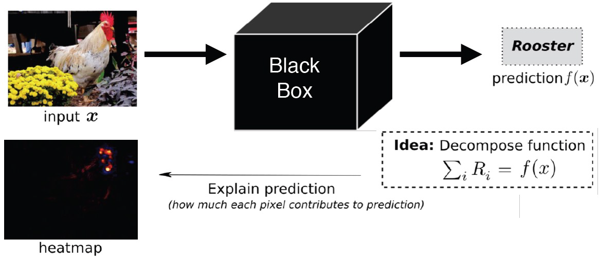
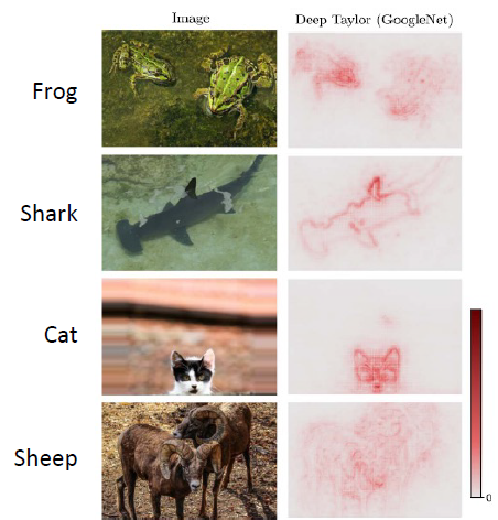
LRP calculates the attribution (i.e., relevance, importance) of each pixel \(i\) in the input image x to the model prediction \(f(\mathscr{x})\)
feature level
LIME
全称 Local Interpretable Model-agnostic Explanations,可以理解为模型的解释器。
"Why Should I Trust You?": Explaining the Predictions of Any Classifier
 - 用户需要信任预测结果:举一个论文中提到的例子,一个医学模型判断病人患病,通过 LIME 算法同时给出病人的病史症状包括喷嚏、头痛等特征,医生利用自己的先验知识,就能更好地借助模型做出决定。

- 建模者需要信任模型:每个算法都需要对模型整体信任度有一定的衡量,意思就是模型是否学到了我们所预期的东西。论文中举出一个文章分类的例子,判断该文章与“基督教“有关还是与”无神论教“有关,分类器本身达到了 90% 的准确率。但是利用 LIME 解释器,发现”无神论教“的重要特征,是”Posting“( 邮件标头的一部分 ),这个词与无神论本身并没有太多的联系。这意味着尽管模型准确率很高,但所学习到的特征是错误的。
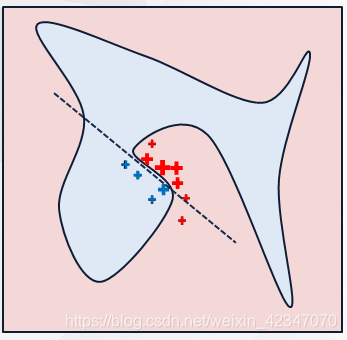
如图所示,红色和蓝色区域表示一个复杂的分类模型(黑盒
SHAP
shapley Values
一群拥有不同技能的参与者为了集体奖励而相互合作。那么,如何在小组中公平分配奖励?

考察一个对象对剩余对象的子集,有什么边际影响。
这才是 Shapley 值背后真正的力量和吸引力。然而,这是有代价的。对于一组参与游戏的 \(n\) 个玩家,你将需要分析 \(2^n\) 个子集才能计算 Shapley 值。
有一些方法可以使计算更加实际可行,在引言中我提到了 SHAP 框架,它的主要优点是,当将 Shapley 值应用于机器学习时,它能够更有效地计算 Shapley 值。
Concept level
!!! note "which high-level concepts are important when a model classifies one class of inputs across the entire dataset? (Global Explanation)"
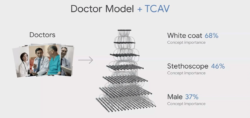
TCAV
- Represent the concept as a vector (referred to as Concept Activation Vector (CAV) 决策边界线的正交向量 )
- Quantify the sensitivity of an image to the CAV vector
- Measure the importance of the concept to multiple images of the same class
ACE
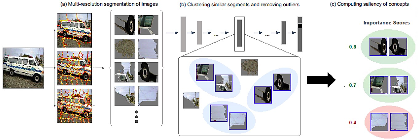
ACE advantage over the TCAV approach: It does not require a manual selection of a set of positive and negative images for a concept
Instance level
prototype & criticism
Prototypes: representative examples of the class
Criticisms: examples of the class that are not well represented by the prototypes
Maximum Mean Discrepancy (MMD) to measure the discrepancy between two distributions, given by
Prototypes
To find prototypes: 1. Start with an empty set of prototypes. 2. While the number of prototypes is below the chosen number $ m $: - For each instance in the dataset, check how much MMD is reduced when the instance is added to the set of prototypes. - Add the data instance that minimizes MMD to the set of prototypes. 3. Return the set of prototypes.
Criticisms
To find criticisms, the following witness function is used: $$ text{witness}(x) = frac{1}{n} sum_{i} k(x, x_i) - frac{1}{m} sum_{j} k(x, z_j) $$ - The witness function evaluates which of two distributions fits the instance $ x $ better.
For a trained black-box model, the predicted classes for the prototypes and criticisms can help to understand the model
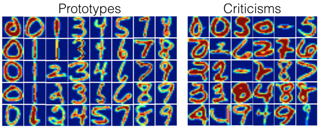 The prototypes represent common way of writing digits, whereas the criticisms
represent outliers and ambiguously written digits
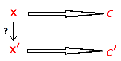
counterfactuals explanation
change the input feature vectors
